Introduction
When most people start Machine Learning, they quickly jump to libraries like scikit-learn. While that is useful in practice, it often skips the most important part — understanding how the algorithm actually works.
This blog documents my learning of Simple Linear Regression, where I deliberately avoided using ready-made models and instead focused on:
- Understanding the mathematics behind Linear Regression
- Deriving the formulas for slope and intercept
- Implementing the algorithm completely from scratch in Python
The intention was simple: learn the logic first, then scale up with libraries later.
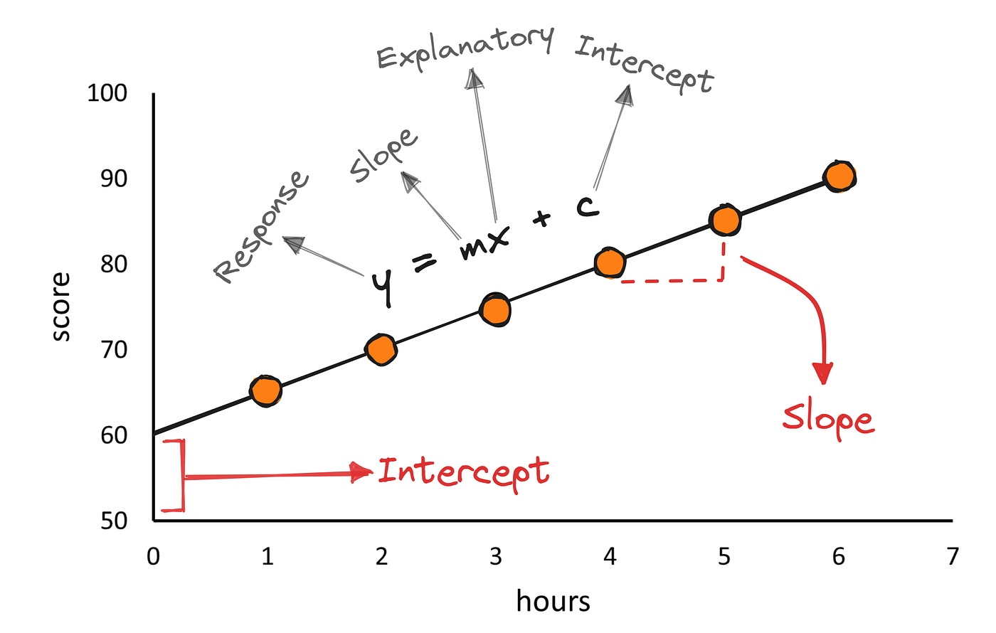
What is Simple Linear Regression?
Simple Linear Regression is a supervised learning algorithm used to model the relationship between two variables:
- An independent variable (X)
- A dependent variable (y)
The model assumes a linear relationship, represented by the equation:
y = mx + b
Here:
- m (slope) represents how much the output changes for a unit change in input
- b (intercept) represents the output value when the input is zero
The entire objective of Linear Regression is to find the best possible values of m and b such that the predicted values are as close as possible to the actual values.
Understanding the Error
For each data point, the prediction error is defined as:
error = actual value − predicted value
If we simply add errors, positive and negative values may cancel each other out. To avoid this and to penalize larger mistakes, we square each error.
This leads to the Least Squares Error, commonly written as:
Σ (yᵢ − (mxᵢ + b))²
The goal of training a Linear Regression model is to minimize this error.
How the Best-Fit Line is Calculated
Instead of guessing values for m and b, we can derive them mathematically by minimizing the error function.
For Simple Linear Regression, the closed-form solutions are:
m = Σ(xᵢ − x̄)(yᵢ − ȳ) / Σ(xᵢ − x̄)²
b = ȳ − m x̄
Where:
- x̄ is the mean of all input values
- ȳ is the mean of all output values
This formula ensures that the resulting line passes through the center of the data and minimizes the total squared error.
Implementing Linear Regression from Scratch
To truly understand the algorithm, I implemented Linear Regression without using any ML libraries.
The implementation follows three core steps:
- Compute the mean of X and y
- Calculate the numerator and denominator for slope (m)
- Compute intercept (b) using the derived formula
Once m and b are known, predictions can be made using the hypothesis equation.
This approach removes the abstraction layer and makes the learning process much more concrete.
Why Building From Scratch Matters
Implementing Linear Regression manually helped me understand:
- Why mean centering is important
- How covariance and variance influence the slope
- How error minimization shapes the final model
More importantly, it built a strong foundation for advanced topics such as:
- Gradient Descent
- Multiple Linear Regression
- Feature Scaling
- Regularization
Attached Reference: Implementation Notes (PDF)
Along with this blog, I have attached a PDF containing my handwritten derivations and Python implementation of Linear Regression from scratch.
This PDF includes:
- Step-by-step logic for calculating
mandb - Python class-based implementation
- Sample predictions on a real dataset
Conclusion
Learning Machine Learning algorithms from scratch provides clarity that libraries alone cannot offer.
Understanding the mathematics behind Linear Regression made the algorithm feel intuitive rather than magical. This experience reinforced an important lesson:
Good ML engineers don’t just use models — they understand them.
Next step in this journey: Gradient Descent and optimization techniques.